
Navigating Databricks Compute Options for Cost-Effective and High-Performance Solutions
- Matt Collins
- Aug 15, 2024
- 9 min read
Updated: Oct 21, 2024
Choosing The Right Cloud Compute For Your Workload
You can use Databricks for a vast range of applications these days. From handling streaming datasets, running Deep Learning models to populating data model fact tables with complex transformations, choosing the correct compute option can seem a lot like a stab in the dark followed by (potentially expensive) trial end error.
You can choose from an incredible range of configurations in the Databricks Compute User Interface.
This variety is comprised of the Virtual Machine (VM) category, size, availability and access mode (also referred to as family).
Determining the right compute choice for you could be answered by the classic answer “it depends”, but this guide aim to inform the decision-making process — both in terms of cost and performance.
Disclaimer: While this article is intended for Databricks Compute, the core concepts are relevant for other using Apache Spark on cloud compute applications, such as in Azure Synapse Analytics.
Contents

Finding a starting point
Before spinning up some personal compute to see what is appropriate for your use case, first break the problem down by the following areas.
Tasks
It is important to understand the task you are performing: if it can be categorised into one of the following areas then you will have clearer guidance on your performance requirements under the hood.
Common tasks are:
Data Analysis
Basic Extract Transform Load (ETL)
Complex ETL
Machine Learning
Streaming Data
This Databricks article has some good insights to requirements for these sorts of tasks.

Data Volume

Next up, think about the Data Volume you’re handling. How many rows are you dealing with, both in terms of expected input and outputs. You might bucket this into “Small”, “Medium” and “Large” initially.
It is worth mentioning that data volume will probably change over time. By frequently reviewing your compute usage and performance, you will get a picture of how to scale clusters over time as and when it is required to do so. More on monitoring later in the article.
Data Complexity
What is the Data Complexity? Does your dataset have nested columns? Are you performing some heavy transformations as part of your processing? Or do you have lots of simple tables that you’re copying from one location to another, possibly including some simple MERGE statements?
This could be categorised as Simple, Medium and Complex.
Future Executions and Implementation
Who/what will be running the task you’re working on? There are a few configuration options we need to consider that are important as to who can use a cluster. If it is non-urgent, and you don’t mind waiting a bit longer for your workload to complete, you can look to using Spot instances, which are available at a cheaper rate.
If it is a hands-off process (such as a notebook executed through a Workflow or other Orchestration Tool), then you’ll look at Job clusters instead of interactive clusters.
This is common as you move from development to production implementations.

Working with the UI
The below screenshot shows the Compute User Interface. Before we think about sizing we can see compute “Families” available.
It is worth adding a disclaimer here that Databricks Serverless Compute has just gone Generally Available. This extends the previously available SQL Warehouses to give users the power of notebooks executing other languages on serverless compute, saving development time and costs from spinning up and turning off compute as and when required. As this is a more hands-off configuration with less administrative control, it will be out-of-scope of this article. More info on enabling this feature and some of the considerations can be found here.
I’ve summarised each of the compute categories as a 1-liner:
All-purpose compute: Interactive compute that users and other tools can use to develop, test and debug executions.
Job compute: Compute only accessible by automated tasks that are started for the task at hand and shutdown after completion.
SQL warehouses: Clusters for SQL-only executions which include Serverless options.
Pools: A collection of idle compute which can be allocated to various clusters for improved availability and execution time.
Policies: This is out-of-scope for this article.
It is worth noting that some options here depend on using a Premium Databricks plan.
We can start to answer some of our burning questions already with this knowledge.
Case 1

If you’re looking for Analytics SQL only workloads (such as using your Semantic Data Model in a Power BI report), then SQL warehouses are a natural choice. The possibility of Serverless means little-to-no start-up time required for any queries that will hit your tables directly is a great benefit for reporting.
Case 2
Developers looking to develop a new data engineering notebook will want to look at all-purpose compute options.
Case 3
Users creating orchestration pipelines (such as Databricks Workflows or Azure Data Factory) will configure Job clusters.
Now that we’re getting a feel for what type of compute to use, we can think about the specifications required. To explore what is available, navigate to the All-purpose compute tab.
All-purpose compute
There’s a lot going on here, so let’s gloss over the options that we are not concerned about in the context here.
Policy: Again, this is out of scope for this article - please refer to the following documentation for some guidance.
Multi-node / Single-node: How many VMs do you want to build your compute cluster from?
Consider the following:
Consider single node for tasks for non-intensive workloads on the smallest cluster size.
Data Analysis tasks perform better on single node clusters.
Machine Learning operations are also suited to single node clusters as many operations cannot be parallelised efficiently.
If you are performing operations of varying resource utilisation, smaller multi-node compute is often cheaper than 1 large single-node machine, due to the ability to scale up and down as needed.

Access mode: Who can use the compute being created, and in what programming languages.
Performance Options
Let’s talk briefly about each of the options that are available.
Databricks runtime version: What version of Spark do you want installed on the cluster, and do you need any Machine Learning libraries pre-installed?
Photon Acceleration: C++ engine which can speed up query performance, for an increased base cost (DBUs). There is a threshold at which using Photon will be make workloads run fast enough to save money, but this is not a guarantee.
Note: If you’ve selected multi-node compute then you will see worker and drive node configuration options. Discussing the breakdown how Spark applications use compute in their operation is out-of-scope of this article, so if you are unsure of the difference between these and their purpose then I recommend Spark: The Definitive Guide, or other documentation and articles available online.
Worker type: The compute category and size available for your worker nodes.
An information tooltip shows that options with local SSDs are recommended for delta-caching. The linked Azure Databricks documentation clarifies this is used for faster reads. The DBUs for Delta-Accelerated spec VMs is slightly higher than standard VMs. As such, if you're running development workloads that do not need faster storage, then consider using standard type VMs.
Min workers: When the cluster starts up, this is how many worker nodes it will initially provision.
Max workers: How many nodes the cluster can scale up to upon utilisation.
Spot instances: Cheap alternative for on-demand compute instances. Compute may be evicted at Cloud Provider’s discretion. As elaborated in this article, these are a great choice for development.
Driver type: The compute category and size of the driver node. Simplest option is to match your Worker type, unless you are performing lots of in-memory operations on the driver node such as returning a large dataset (e.g when using df.collect() in PySpark) for operations which require more memory than required on your driver node. This is common in Data Analysis where we want to view the results of a DataFrame for Exploratory Data Analysis (EDA) and visualisation, so a larger driver node (or large Single Node set-up) is best here.
Enable autoscaling: If true, then the compute will scale out nodes as required. If false, then the compute has a fixed number of nodes, even if they are idle. More info here.
Terminate after…: After how many minutes of being completely idle does the cluster shutdown. I recommend keeping this low to avoid fees for idle cluster activity.
Node Categories

Upon expanding the drop-down list for the Worker type, a rather-overwhelming number of VM specifications appear. This is broken down into Categories:
General purpose (Including Delta Cache accelerated, Standard and HDD options)
Standard Azure VM SKUs
Memory optimised (Including Delta Cache accelerated, Standard and HDD options)
High Memory to Core ratio
Good for large-scale data processing and Machine Learning
Storage optimised (Including Delta Cache accelerated option)
Faster storage configuration
Great for query-intensive workloads
Compute optimised (Standard option)
Higher Core to Memory ratio
Suitable for streaming workloads
May be a cheaper option if your activities are not-memory demanding
Confidential (Encompasses General purpose and Memory optimised categories)
Use AMD Secure Encrypted Virtualization to protect data with full VM encryption
Limited VM sizes and configurations available
GPU accelerated
For Deep Learning
Availability limited to certain regions
Translating these to our Tasks and complexities mentioned previously, we can draw the following diagram. Please find the full animated version at the end of this post!

Node Sizes

Compute size examples used in this article are from Azure Databricks. AWS and GCP interfaces may differ to correspond with Cloud Provider VM options.
Choose a node size corresponds the size of the underlying VM. These correspond with Virtual Machines you can create yourself within the Azure Portal.
If you’re not too hot on Virtual Machine configurations, ignore the “Standard_*” names for now and look at the Memory and Cores available for each VM. At a very quick glance, you will notice that the ratios between Memory and Cores change depending on the node category, with a higher memory to core ratio for Memory Optimised VMs and a lower memory to core ratio for Compute Optimised — allowing you to be more cost effective when scaling out the hardware you require. This seems logical given the categories we’ve talked about just before this.
With that in mind, let’s break down the naming convention, again remembering that this refers to Azure VMs. This documentation should be a good reference point.

More info on the Azure VM naming can be found here.
A complete list of the different instance sizes available for virtual machines in Azure is available here.
You won’t need to consider the VM family too much if you understand which node category is appropriate for your workload.
Key points to consider are the following:
The number of CPUs is the number of cores for task parallelisation, and corresponds to the processing power available.
Ensure you have enough memory on the Driver node if you are running any commands (like df.collect() ) which return results you may wish to display.
The local storage options are not as essential to understand either, unless you’re facing some complex storage requirements as part of your operations.
As a rule of thumb, more recent versions will have additional features and performance improvements available.
The DBUs for VMs (within the same category) of the same size is generally the same, so you won’t see a pricing difference here. At the more demanding end of the scale you may see cost differences between different versions/storage options
Determining the correct node size can be complicated and may change over time. If you know how much data you are processing then you can use some optimisation details to calculate the number of core you need to run a task fully parallel. Of course, you may want to consider the cost-performance trade-off in your decision.
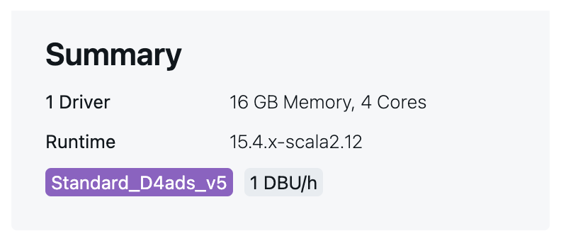
Summary box
Review the details captured in the summary box to ensure your config looks right and that the DBU/h falls into your expected value.

Other Notes
This configuration can be achieved through the CLI, Terraform and Bicep, if preferred.
Review performance metrics to understand bottlenecks.
High-utilisation is good! If you're only hitting 10% of resource utilisation, you are probably over-paying and can look to down size and save a bit of money.
If using All-purpose clusters, reduce the overlap of tasks this compute shares. Do not assign a single cluster for multiple purposes with different requirements.
Putting Everything Together
Trying to condense the entire article into a single cheat-sheet is quite difficult, but I’ve attempted this through the visuals below:
Final Thoughts
This article attempts to bring together all of the considerations required when configuring Databricks compute clusters for different use cases.
Hopefully after reviewing the content, you have an understanding of the type of cluster to use, what sizes to consider and what options you can use to be cost effective.

The next natural step to evaluate you’ve made an appropriate choice is to set up monitoring.
Depending on the granularity of monitoring you wish to perform, you can take a couple of approaches:
Add Tags to your Compute resources and monitoring through the Azure Spend Portal.
If you’ve got Unity Catalog enabled on your workspace, you can query system tables to get the information on the metrics you want to track, and not just high-level spend trends over time. This gives a breakdown tailored to you that is not possible through default Azure monitors.
There is a great Power BI template you can use on top of the system tables to leverage some useful pre-built visuals.
If you have any thoughts or questions on this, please reach out and ask!
Thanks

Comments